Our goal here is to gain a quantitative understanding of how the membrane potential of a simple Resistor-Capacitor (RC) model neuron changes over time in response to an external current injection.
Why is it important to consider our simple neuron’s response to current input? We ultimately want to understand quantitatively how neurons interact with and causally influence each other. When one neuron influences another it most often does it by releasing a neurotransmitter which binds a receptor on a post-synaptic neuron and opens an ion channel - this is basically a current injection! We’ll start by considering the simplest possible case - a neuron which is essentially just a closed membrane, with no leaks, receptors, or channels.
The Capacitor Neuron
What is a Capacitor Neuron?
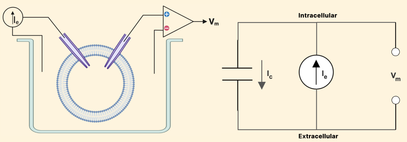
Let’s with that simplest of cases: a closed neural membrane in a salt solution, where we record the membrane potential, \(V_m\), and inject some amount of current, \(I_e\) (e for external current). We will call this a capacitor-neuron, and Figure 1 shows what our simple setup and corresponding equivalent circuit would look like:
Figure 1: Left: experimental setup, Right: a circuit model of a simple capacitor neuron
Why is a neuron like a capacitor?
Why exactly are we referring to this simple case as a ‘capacitor?’ We see in Figure 1 that there is a capacitive current, \(I_C\), flowing out of our cell.
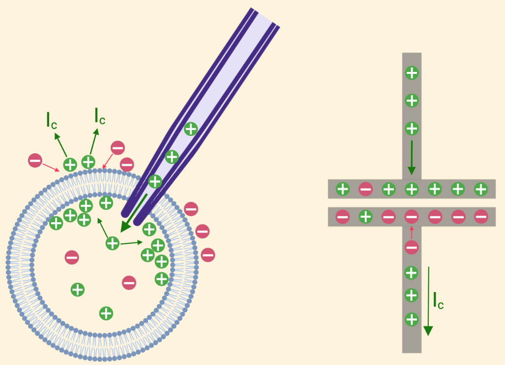
So what exactly is this capactive current? Since there is no hole in our membrane, how is there current flowing anywhere but through our electrode? Think about what exactly happens at the ionic level when we inject current into our neuron - we are essentially pumping positive ions into the cell, which leads to a buildup of excess positive charge inside our cell. This excess positive charge may be attracted to negative charges outside the membrane which will lead to further buildup of positive charge along the inside of the neuronal membrane. When this happens, the positive charges on the outside of the membrane will be strongly repelled by the large buildup of positive charge on the inside, and will move away from the membrane. This movement of positive charge away from the membrane is the source of the capactive current, and can be seen in Figure 2 in a neuron (left), and traditional capacitor (right).
Figure 2: Capactive Current in a Neuron and a Capacitor
Principle: The Neuronal membrane has properties similar to a capacitor.
How Does the Capacitor-Neuron Respond to a Current Injection?
We know from Kirchoff’s Law that the current flowing into our cell must equal the current flowing out, so we can say the following: \[I_e = I_c \tag{1.1}\]
We also know that a current is just a change in charge over time, \(\frac {dQ} {dt}\), and we know that a charge imbalance is simply equal to the corresponding voltage difference scaled by the capacitance, in other words: \[ \Delta Q = C \Delta V \tag{1.2}\]
Making that simple substitution, we can now modify equation (1.1) and describe our injected current in the following way: \[I_e(t) = C \frac {dV_{m}(t)} {dt} \tag{1.3}\]
We would like to isolate the variable \(V_m\) here knowing how a neuron ‘responds’ to current injection means knowing (at least) what happens to its membrane potential. To do so, we will integrate equation (1.3) with respect to time to get: \[V_{m}(t) = V_0 + \frac 1 C \int_{0}^{t} I_{e}(t) dt \tag{1.4}\]
This means that the membrane potential at time \(t\) is equal to the initial voltage, \(V_0\), plus the integral of the injected current scaled by the inverse of the capacitance. Since current is simply charge over time, when we integrate with respect to time, we are left only with a change in charge, \(\Delta Q\), and since \(\Delta V = \frac {\Delta Q} C\), equation (1.4) is simply saying that our membrane potential at time \(t\) is equal to the initial voltage plus the change in voltage.
Now we have all the tools we need to describe how the membrane potential of our simple capacitor-neuron responds to our current injection. We know from equation (1.3) how to describe the way in which our voltage changes with respect to time in response to the injected current: \[\frac {dV_{m}(t)} {dt} = \frac {I_e(t)} {C} \tag{1.3}\]
And we know from equation (1.4) that our membrane voltage at time \(t\) is equal to our initial voltage plus the change in voltage. If we multiply the way in which \(V_m\) changes with respect to time (equation 1.3) by the amount of time it does so, we can get the total change in voltage and subsitute it into equation (1.4) to get: \[V_{m}(t) = V_0 + \frac {I_e(t)} {C} t \tag{1.5}\]
We can write this equation in python and add a few lines of code to plot the membrane potential over time in reponse to a current injection, which allows us to answer our question: the capacitor-neuron is just integrating the injected current over time!
Code
import numpy as npfrom plotly.subplots import make_subplotsimport plotly.graph_objects as goimport plotly.io as pioimport plotly.io as piopio.renderers.default ="plotly_mimetype+notebook_connected"em_xaxis = go.layout.XAxis(color='black', gridwidth=0.8, gridcolor='#D8D9D9', zerolinewidth=1.5, zeroline=False)em_yaxis = go.layout.YAxis(color ='black', gridwidth=0.8, gridcolor='#D8D9D9', zerolinewidth=1.5, zeroline=False)pio.templates['plotly_em'] =dict(layout=go.Layout( plot_bgcolor='#fff4dc', paper_bgcolor='#fff6e3', xaxis=em_xaxis, yaxis=em_yaxis, ))pio.templates.default ="plotly_em"green ='#157a10'blue ='#2b7de1'red ='#d61717'
Code
def capacitor_current_response(length, buffer, amps=1):"response of capacitor neuron to current injection, assumes constant current defined by 'amps' " cap=1 v_o =0 buff = np.zeros(buffer+1) currents = np.ones(length+1)*amps currents = np.append(buff, currents) currents = np.append(currents, buff) times = (buffer)*2+ length +1 times = np.arange(times) current_times = np.insert(times, [buffer, buffer+length], [buffer, buffer+length]) membrane_potentials = [] stim_times = np.arange(0, length+1)for t in stim_times: v_m = v_o + (amps/cap)*t # equation (1.5) membrane_potentials.append(v_m) mp = np.insert(membrane_potentials, 0, np.zeros(buffer+1)) mp = np.append(mp, np.ones(buffer+1)*mp[-1:])return current_times, currents, mptimes, current, v_m = capacitor_current_response(6, 2)fig = make_subplots(rows=2, cols=1, shared_xaxes=True)fig.add_trace(go.Scatter(x=times, y=v_m, mode='lines', line=dict(color='#157a10', width=4)), row=1, col=1)fig.add_trace(go.Scatter(x=times, y=current, mode='lines', line=dict(color='#2b7de1', width=4)), row=2, col=1)fig.update_layout(height=600, width=800, title_text="Membrane Response to Current Injection", showlegend=False)fig.update_yaxes(showticklabels=False, title_text="Membrane Potential", row=1, col=1)fig.update_yaxes(showticklabels=False, title_text="Current", row=2, col=1)fig.update_xaxes(title_text="Time", row=2, col=1)fig.show()
Figure 3: A capacitor neuron integrates the injected current over time
The Resistor-Capacitor Neuron
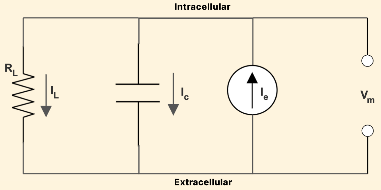
Let’s say that we poke a hole in the membrane of our neuron from figure 1. We’ll call this hole a “leak,” and for now can think of it as not specific for any ion. This hole hole allows ions to leak out (i.e. allows some current to flow), with some resistance value - this where the ‘resistor’ part of the name comes from. Figure 4 shows the modified circuit model of our RC-neuron, with the leak resistance and leak current added:
Figure 4: Circuit model of a simple RC-neuron
How Does the RC Neuron Respond to Current Injection?
Again, the current coming into the cell must equal the current flowing out: \[I_e = I_c + I_L \tag{1.6}\]
We can descibe our leak current using Ohm’s Law, \(I_L = \frac {V_m} {R_L}\), which we can then substitute into equation (1.6) and combine with equation (1.3) to obtain: \[I_e = \frac {V_m} {R_L} + C \frac {dV_m} {dt} \tag{1.7}\]
Some basic rearrangement gives us: \[I_e R_L = V_m + R_L C \frac {dV_m} {dt} \tag{1.7}\]
If our simple capacitor-neuron from figure 1 served to integrate the injected current over time, how does this cell behave differently? We know it cant simply integrate, because there is a leak, so when we turn the current off, something different is going to happen.
Let’s think about what would happen if we were to inject some current into our RC-Neuron, and then wait a very long time, until the membrane potential reaches some steady-state, which we will call \(V_{\infty}\).
By definition, when this is the case, \(V_m\) is not changing, so we can set \(\frac {dV_m} {dt}\) to zero. In this condition, we refer to the membrane potential as \(V_{\infty}\), and so from equation (1.7) we can see: \[V_{\infty} = I_e R_L \tag{1.8}\]
In other words: \(V_{\infty}\) is just defined by Ohm’s law.
Since we know that the units of Resistance*Capacitance is time (seconds), we will the refer to the quantity \(R_L C\) (the ‘RC’ in ‘RC-neuron’) as the time constant, \(\tau\). Making a substituition into equation (1.8) using what we know from equation (1.7), we get the following very important equation, whose form we will utilize consistently: \[V_m + \tau \frac {dV_m} {dt} = V_{\infty} \tag{1.9} \]
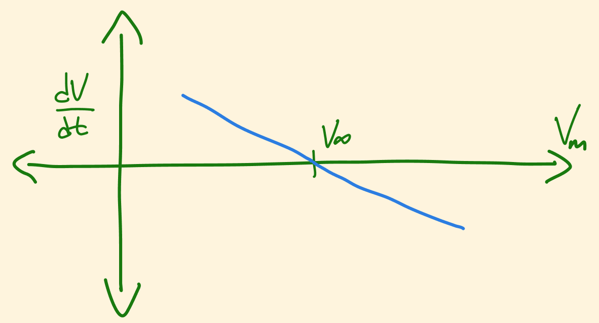
Which can be rearranged to be: \[\frac {dV_m} {dt} = \frac {-1} {\tau} (V_m - V_{\infty}) \tag{1.9} \]
This should make it clear that if \(V_m\) is less than \(V_{\infty}\), then \(\frac {dV_m} {dt}\) is going to be positive, and vice-versa. This becomes particularly obvious when looking at a simple sketch plot of \(V_m\) vs \(\frac {dV_m} {dt}\):
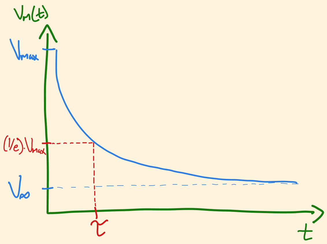
Another way of saying this is that \(V_m\) is always approaching \(V_{\infty}\)! The next logical question is: if \(V_m\) is approaching \(V_{\infty}\), in what way does it get there? We can see from figure 5 that the rate at which \(V_m\) approaches \(V_{\infty}\) is proportional to how far away \(V_m\) is from \(V_{\infty}\) - i.e. it doesn’t get there in a linear fashion, but according to some exponential function:
Figure 6: \(V_m\) approaches \(V_{\infty}\) according to an exponential function
Summing this all up, we are essentially saying the following: if you would like to know the distance that \(V_m\) is from \(V_{\infty}\) at any given time, you simply take the initial distance scaled by an exponential decay function – the distance between \(V_m\) and \(V_{\infty}\) decays exponentially.
Putting those words into math, we arrive at another crucial equation: \[V_{m}(t) - V_{\infty} = (V_0 - V_{\infty})e^{\frac {-t} {\tau}} \tag{1.10}\]
And again, we can use python to represent that equation and plot it (this time using realistic values you may see in actual neurons):
Code
def pulse_on(plm=8, v_o=0):"This function calculates the response of an RC-neuron when the pulse is turned on" cap=1e-10 resistance =1e8 tau = cap*resistance amps=0.5e-6 pulse_length = plm*tau times = np.arange(0, pulse_length+.001, .001) vm_vals = [] vinf_vals = []for t in times: v_inf = resistance*amps # equation (1.8) diff = (v_o - v_inf)*np.exp(-t/tau) # equation (1.10) v_m = diff + v_inf vm_vals.append(v_m) vinf_vals.append(v_inf) currents = np.ones(len(times))*ampsreturn times, currents, vinf_vals, vm_valsdef pulse_off(tm, c, vinf_vals, vm_vals):"This function calculates the response of an RC-neuron when the pulse is turned off" cap=1e-10 resistance =1e8 tau = cap*resistance amps=0 v_o = vm_vals[-1] times = np.arange(0, 0.1, .001)for t in times: v_inf = resistance*amps # equation (1.8) diff = (v_o - v_inf)*np.exp(-t/tau) # equation (1.10) v_m = diff + v_inf vm_vals.append(v_m) vinf_vals.append(v_inf) currents = np.zeros(len(times+1)) times = times+tm[-1] times = np.append(tm, times) currents = np.append(c, currents)return times, currents, vinf_vals, vm_valsdef pulse_buffer(t, c, vi, vm, v_o=0):"This function just serves to add a bit of time before the current is injected to make the plot look better" length =.03 t = t+length buf_t = np.arange(0, length+.001, .001) times = np.append(buf_t, t) buff_zeros = np.zeros(len(buf_t)) buff_vo = np.ones(len(buf_t))*v_o current = np.append(buff_zeros, c) vi = np.append(buff_zeros, vi) vm = np.append(buff_vo, vm)return times, current, vi, vmdef rc_pulse_response(plm=8, v_o=0): t, c, vi, vm = pulse_on(plm=plm, v_o=v_o) t, c, vi, vm = pulse_off(t, c, vi, vm) times, currents, vi, vm = pulse_buffer(t, c, vi, vm, v_o=v_o) times *=1000return times, currents, vi, vmtimes, current, v_inf, v_m = rc_pulse_response(plm=10)fig = make_subplots(rows=3, cols=1, shared_xaxes=True)fig.add_trace(go.Scatter(x=times, y=v_m, mode='lines', line=dict(color=green, width=4)), row=1, col=1)fig.add_trace(go.Scatter(x=times, y=v_inf, mode='lines', line=dict(color=blue, width=4)), row=2, col=1)fig.add_trace(go.Scatter(x=times, y=current, mode='lines', line=dict(color=red, width=4)), row=3, col=1)fig.update_layout(height=500, width=800, title_text="Membrane Response of RC-Neuron to Current Injection", showlegend=False)fig.update_yaxes(showticklabels=True, title_text="Membrane Potential", row=1, col=1)fig.update_yaxes(showticklabels=True, title_text="V-infinity", row=2, col=1)fig.update_yaxes(showticklabels=True, title_text="Current", row=3, col=1)fig.update_xaxes(title_text="Time (ms)", row=3, col=1)fig.show()
Figure 7: RC-neuron response to current pulse: an exponential path toward a steady-state potential
The RC Neuron is a Low-Pass Filter
We now have an answer to our question of how the RC-neuron responds to a current pulse: the distance between the membrane potential and a steady state solution of the membrane potential shrinks exponentially (Figure 7).
This is important. But what does that actually mean? What is the actual functional significance of that - i.e. what unique thing does it allow our neuron to do?
Our simple capacitor-neuron was just an integrator - it integrated the injected current over time (Figure 3). While the RC-neuron is doing some integration, it is not really doing it in the same exact way, and there is something else happening.
Let’s take a look at what happens when we vary the duration of our current injection. I’ll do that in Figure 8, where we can see the response to current pulses that are different multiples of \(\tau\). Importantly, I’m using the same exact math as that in Figure 7, and just varying how long the current is applied.
Reminder: \(\tau\) has units seconds and in this case represents the amount of time it takes for the distance between \(V_m\) and \(V_{\infty}\) to shrink to \(1/e\) of its initial value (see Figure 6 and check the values for yourself in Figure 7)
Figure 8: The response of an RC-neuron is dependent on the length of the current pulse
When the current injection is long (a high multiple of \(\tau\)), the membrane potential reaches \(V_{\infty}\) - we can think of this as a ‘strong’ response. When the current injection is very brief, the membrane potential does not reach \(V_{\infty}\), which we can think of as a ‘weak’ response. These properties - responding strongly to long/infrequent things, and responding weakly to brief/frequent things - describe a low-pass filter. If a brief current pulse comes along (say a bit of transmitter is released at a synapse and a few ion channels are opened), the neuron acts as a low-pass filter by not reponding. And for good reason - the release of small amounts of transmitter at a single synapse may just be a random event, and the neuron shouldn’t want to respond strongly to that. On the other hand, if a bunch of synapses all have a lot of transmitter released onto them, from a number of presynaptic cells, that probably signals something very important that the post-synaptic neuron would want to respond to. The low-pass filtering qualities we’ve described in this section are what give neurons that ability.
To make the point one last time, here is a plot of the response strength of our RC-neuron (as a fraction of \(V_{\infty}\) vs the duration of the current pulse):
Code
import plotly.express as pxpulse_lengths = np.arange(0.1, 6, 0.1)def response_fraction(plm=8, v_o=0):"This function calculates the response of an RC-neuron when the pulse is turned on" cap=1e-10 resistance =1e8 tau = cap*resistance amps=0.5e-6 pulse_length = plm*tau v_inf = resistance*amps diff = (v_o - v_inf)*np.exp(-pulse_length/tau) v_m = diff + v_infreturn v_m/v_infresponse_fracs = []for i in pulse_lengths: rf = response_fraction(plm=i) response_fracs.append(rf)fig = px.scatter(x=pulse_lengths, y=response_fracs, title="The RC-Neuron is a Low-Pass Filter", color_discrete_sequence=[green, blue, red],labels={"x": "Pulse Length (as a multple of tau)", "y": "Maximal Vm Reponse (as a fraction of V-infinity)"})fig.update_xaxes(zeroline=True)fig.update_yaxes(zeroline=True)fig.show()
Figure 9: An RC-neuron acts as a low-pass filter, and reponds most effectively to a current pulse that is long/slow
Does \(\tau\) Depend on a Neuron’s Size?
We know that \(\tau\) is a function of resistance and capacitance, so let’s think about those quantities in terms of a cell’s size.
First, we know \(\tau = R_L C\), and since the inverse of resistance is conductance, we can rewrite that as: We also know that the inverse of resistance is conductance, which means we can write: \[\tau = \frac {C} {G_L} \tag{1.11}\]
We also know that conductances in parallel add together, so if a neuron has a bunch of ion channels on it’s membrane, those conductances all add up to get the total conductance. We can say the same about capacitance.
This means we can calculate the conductance of a cell by multiplying the total area of the membrane, \(A\), by the conductance per unit area (or ‘specific leak conductance’), \(g_L\). We can do the same with capcitance, using the specific membrane capacitance, \(c_m\). We can then substitute these values into equation (1.11) to get:
\[\tau = \frac {c_m A} {g_L A} \tag{1.12}\]
Which easily simplifies to: \[\tau = \frac {c_m} {g_L} \tag{1.12}\]
As should now be apparent, \(\tau\) depends not at all on the size of the cell or area of it’s membrane - only on the specific conductance and capacitance properties per unit area of the membrane. \(\tau\) is only a property of the membrane, and not of the cell itself.